
R is a highly capable GIS tool, thanks to the sf package. In this post I am going to show you how you can use sf with openly available data to calculate catchment areas and population sizes, and then how to calculate travel time isochrones with osrm.
Firstly, I have prepared a dataset containing the 23 A&E departments that are Adult Major Trauma Centres (MTCs) in England and Wales. This dataset is an sf object which contains a special column called geometry - this column contains the locations of the hospitals. The data is sourced from this, the Organisation Data Service (ODS) and the NHS Postcode Database.
When we print this table out we get a bit of information telling us how many features (rows) and fields (columns) there are, along with what the type of the geometry is (in this case, we have points). We also get the “bounding box” (bbox) - this is like a rectangle that encloses all of our geometries. Finally, we get the coordinate reference system (CRS) that is being used.
Below this we see a table of data - like any other dataframe in R.
major_trauma_centres <- read_sf(
paste0(
"https://gist.githubusercontent.com/tomjemmett/",
"ac111a045e1b0a60854d3d2c0fb0baa8/raw/",
"a1a0fb359d1bc764353e8d55c9d804f47a95bfe4/",
"major_trauma_centres.geojson"
),
agr = "identity"
)
major_trauma_centresSimple feature collection with 23 features and 2 fields
Attribute-geometry relationships: identity (2)
Geometry type: POINT
Dimension: XY
Bounding box: xmin: -4.113684 ymin: 50.41672 xmax: 0.1391145 ymax: 54.98021
Geodetic CRS: WGS 84
# A tibble: 23 × 3
name org_id geometry
<chr> <chr> <POINT [°]>
1 ADDENBROOKE'S HOSPITAL RGT01 (0.1391145 52.17374)
2 DERRIFORD HOSPITAL RK950 (-4.113684 50.41672)
3 HULL ROYAL INFIRMARY RWA01 (-0.3581464 53.74411)
4 JAMES COOK UNIVERSITY HOSPITAL RTDCR (-1.214805 54.55176)
5 JOHN RADCLIFFE HOSPITAL RTH08 (-1.219806 51.76387)
6 KING'S COLLEGE HOSPITAL (DENMARK HILL) RJZ01 (-0.09391574 51.46808)
7 LEEDS GENERAL INFIRMARY RR801 (-1.551744 53.80145)
8 NORTHERN GENERAL HOSPITAL RHQNG (-1.455966 53.4098)
9 NOTTINGHAM UNIVERSITY HOSPITALS NHS TRUST -… RX1RA (-1.185957 52.9438)
10 QUEEN ELIZABETH HOSPITAL RRK02 (-1.938476 52.45318)
# ℹ 13 more rowsThis dataframe can be used like any other dataframe in R, for example, we can use dplyr to filter rows out we aren’t interested in, or join to another dataframe to bring in extra information.
For example, we can load the LSOA population estimates and join it to the LSOA boundaries file from the ONS geoportal. If you aren’t familiar with Output Areas see the ONS Census Geography documentation.
First, let’s load the population estimate file.
# download the LSOA population estimates from ons website: for some reason they
# provide this download as an excel file in a zip file, so we need to download
# the zip then extract the file, but we don't need to keep the zip after. withr
# handles this temporary like file for us
if (!file.exists("SAPE22DT2-mid-2019-lsoa-syoa-estimates-unformatted.xlsx")) {
withr::local_file("lsoa_pop_est.zip", {
download.file(
paste0(
"https://www.ons.gov.uk/file?uri=/peoplepopulationandcommunity/",
"populationandmigration/populationestimates/datasets/",
"lowersuperoutputareamidyearpopulationestimates/mid2019sape22dt2/",
"sape22dt2mid2019lsoasyoaestimatesunformatted.zip"
),
"lsoa_pop_est.zip",
mode = "wb"
)
unzip("lsoa_pop_est.zip")
})
}
lsoa_pop_estimates <- read_excel(
"SAPE22DT2-mid-2019-lsoa-syoa-estimates-unformatted.xlsx",
"Mid-2019 Persons",
skip = 3
) %>%
select(LSOA11CD = `LSOA Code`, pop = `All Ages`)
head(lsoa_pop_estimates)# A tibble: 6 × 2
LSOA11CD pop
<chr> <dbl>
1 E01011949 1954
2 E01011950 1257
3 E01011951 1209
4 E01011952 1740
5 E01011953 2033
6 E01011954 2210Now we can load the boundary data and join to our population estimates.
lsoa_boundaries <- read_sf(
httr::modify_url(
"https://services1.arcgis.com",
path = c(
"ESMARspQHYMw9BZ9",
"arcgis",
"rest",
"services",
"LSOA_Dec_2011_Boundaries_Generalised_Clipped_BGC_EW_V3",
"FeatureServer",
"0",
"query"
),
query = list(
outFields="*",
where="1=1",
f="geojson"
)
)
) %>%
# there are other fields in the lsoa data, but we only need the LSOA11CD field
select(LSOA11CD) %>%
inner_join(lsoa_pop_estimates, by = "LSOA11CD") %>%
# this helps when combining different sf objects and gets rid of some messages
st_set_agr(c(LSOA11CD = "identity", pop = "aggregate"))We can now use ggplot to create a simple plot showing the populations of the LSOAs and add points to show the MTCs.
ggplot() +
# first plot the lsoa boundaries and colour by the population
geom_sf(data = lsoa_boundaries, aes(fill = pop), colour = NA) +
geom_sf(data = major_trauma_centres) +
scale_fill_distiller(type = "div", palette = "Spectral",
# tidy up labels in the legend, display as thousands
labels = number_format(accuracy = 1e-1, scale = 1e-3, suffix = "k")) +
theme_void() +
theme(legend.position = c(0, 0.98),
legend.justification = c(0, 1)) +
labs(fill = "Population (thousands)")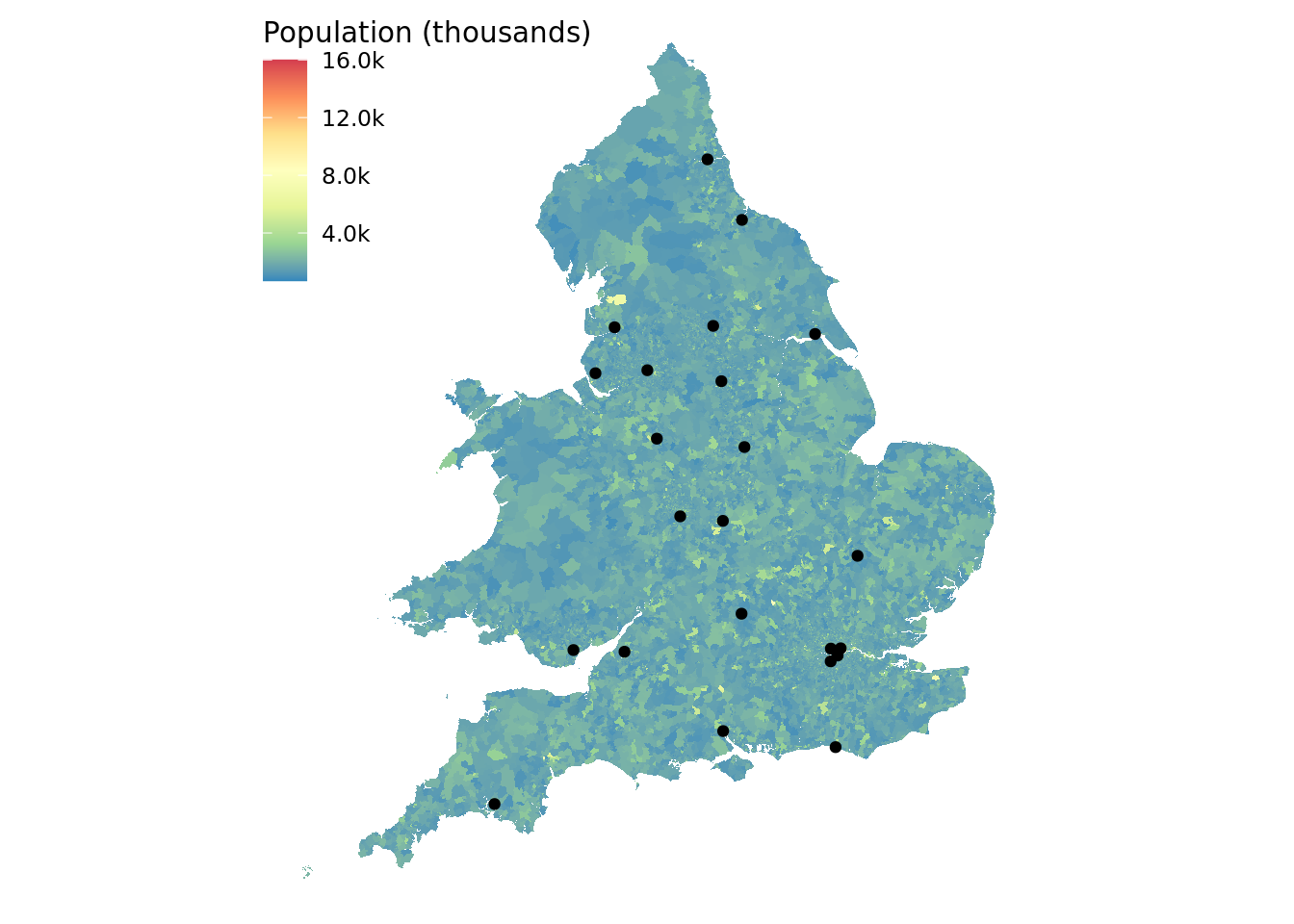
We can now try to calculate the population estimates for each of the MTCs. We can take advantage of {sf} to perform a spatial join between our two datasets. A spatial join is similar to a join in a regular SQL database, except instead of joining on columns we join on geospatial features.
In this case we want to take each LSOA and find which MTC it is closest to, so we can use the st_nearest_feature predicate function with st_join. This will give us a dataset containing all of the rows from lsoa_boundaries, but augmented with the columns from major_trauma_centres.
We can then use standard dplyr functions to group by the MTC name and org_id fields, and calculate the sum of the pop column.
sf is clever - it knows that when we are summarising a geospatial table we need to combine the geometries somehow. What it will do is call st_union and return us a single geometry per MTC.
One thing we need to do before joining our data though is to transform our data temporarily to a different CRS. Our data currently is using latitude and longitude in a spherical projection, but st_nearest_points assumes that the points are planar. That is, it assumes that the world is flat. This can lead to incorrect results.
But, we can transform the data to use the British National Grid. This instead specifies points as how far east and north from an origin. This has a CRS number of 27700. Once we are done summarising our data we can again project back to the previous CRS (4326). This article explains these numbers in a bit more detail.
mtcv_pop <- lsoa_boundaries %>%
st_transform(crs = 27700) %>%
# assign each LSOA to a single, closest, MTC
st_join(
st_transform(major_trauma_centres, crs = 27700),
join = st_nearest_feature
) %>%
# now, summarise our data frame based on MTCs to find the total population
group_by(name, org_id) %>%
# note: summarise will automatically call st_union on the geometries
# this gives us the lsoas as a combined multipolygon
summarise(across(pop, sum), .groups = "drop") %>%
st_transform(crs = 4326)We can now visualise this map. This time we will use the leaflet package to create an interactive html map.
First we need a function for colouring the areas.
pal_fun <- colorNumeric("Spectral", NULL, n = 7, reverse = TRUE)As this is an interactive map we can add popups to the areas to make it easier to identify which MTC we are looking at and to show us the estimated population.
p_popup <- glue_data(mtcv_pop,
"<strong>{name}</strong> ({org_id})",
"Estimated Population: {comma(pop)}",
.sep = "\n")Now we can create our map
mtcv_pop %>%
leaflet() %>%
# add the areas that have been assigned to each MTC
addPolygons(stroke = TRUE,
color = "black",
opacity = 1,
weight = 1,
fillColor = ~pal_fun(pop),
fillOpacity = 1,
popup = p_popup) %>%
# add markers for the MTCs
addCircleMarkers(data = major_trauma_centres,
color = "black",
stroke = TRUE,
fillColor = "white",
weight = 1,
radius = 3,
opacity = 1,
fillOpacity = 1) %>%
setMapWidgetStyle(list(background= "white"))This method certainly is not perfect. For example, we can see that the closest MTC for a large part of Somerset is Cardiff, but in order to reach Cardiff you need to cross the Bristol Channel! Not so easy by a Land Ambulance!
A better approach would be to use some method to calculate travel time from each LSOA to the MTCs, an example of using the Google Maps Travel Time API is covered here. However, as a quick and dirty approach this method doesn’t produce too bad results.
Comments from WordPress site publishing Mike Dunbar
7 June 2021
Hi Tom, interestingly something has gone wrong with the isochrone data for Derriford Hospital: on the map, Derriford is within the 30-60 minute zone for itself, as is the whole of Plymouth and towns close to the A38 such as Ivybridge, South Brent and Buckfastleigh. Yet large parts of presumably remote Dartmoor are in the 0-30 minute zone! Tom Jemmett
9 June 2021
Hi Mike! Interesting… the issue is with the resolution of the isochrones. For whatever reason osrm returns something a bit odd for this hospital! Try the code chunk below, may take a few minutes to run as you tweak the res argument. 50 seems to be a good balance. Leaving res off was what was used in the blog post, though adding in res = 30 explicitly seems to give me different results! suppressPackageStartupMessages({ library(tidyverse) library(sf) library(osrm) library(leaflet) library(leaflet.extras) }) deriford <- c(-4.113684, 50.41672) deriford_iso <- osrmIsochrone(deriford, breaks = seq(0, 150, by = 30), returnclass = “sf”, res = 50) %>% mutate(time = factor(paste0(“[”, min, “,”, max, “)”))) pal <- colorFactor(viridis::viridis(length(levels(deriford_iso\(time))), levels(deriford_iso\)time)) leaflet() %>% addTiles() %>% addPolygons(data = deriford_iso, fillColor = ~pal(time), color = “#000000”, weight = .5, fillOpacity = 0.5, popup = ~time) %>% addMarkers(lng = deriford[[1]], lat = deriford[[2]]) Spatially weighted averages in R with sf | WZB Data Science Blog
1 July 2021
[…] example as circular regions around the points or as Voronoi regions. Additionally, you may consider nearest-feature-joins or travel time isochrones. Which option is more appropriate depends on your […] Nathan Thomas
12 October 2021
Fascinating work Tom! How easy is it to apply this approach to services other than MTCs - is all that’s needed just a geojson file containing the service locations, or does the file need to be formatted in a certain way? Tom Jemmett
19 October 2021
you should be able to just replace the mtc sf object with some other set of points and it should just work! You could run into runtime issues… I only tried it with the relative small set of mtc’s, if you were to replace this with GP practices it could explode and run for a very long time. You could always try tweaking the size of the isochrones to limit the results! :-) Nathan Thomas
2 November 2021
Cool, thanks! Will give it a try when time allows. Deon Ware
20 December 2022
Very well presented. Every quote was awesome and thanks for sharing the content. Keep sharing and keep motivating others.
Back to top