Using R to create column charts featuring 95% confidence intervals
Statistics
tidyverse
ggplot2
Public Health
Author
Daniel Weiand
Published
January 5, 2022
Modified
July 27, 2024
Daniel Weiand – Consultant Medical Microbiologist – Newcastle upon Tyne NHS Foundation Trust
Hello!
This is my first blog post for the NHS R Community, which I stumbled across in the course of my work as a consultant medical microbiologist at Newcastle upon Tyne Hospitals NHS Foundation Trust.
At work, I’ve been trying to use R to create column charts featuring 95% confidence intervals. I approached the friendly people on the NHS R Community’s Slack channel for further information and guidance.
I must add here that the Community’s Slack channel has been extremely helpful to me, as a novice R user, in solving some of the issues I’ve experienced, and highlighting R packages of potential interest. This is the first time I’ve tried to create a ReprEx and now I understand why people love (?) the mtcars database as much as they do!
Step 1: Calculate some summary statistics
I wanted to calculate some summary statistics, including the mean, and standard error or 95% confidence intervals.
Initially I came across the summary() function of Base R, which is helpful as it calculates the Min., 1st Qu., Median, Mean, 3rd Qu., and Max.
However, the summary() function of {base} R does not calculate either the standard error or the 95% confidence intervals:
      mpg             cyl             disp             hp
 Min.   :10.40   Min.   :4.000   Min.   : 71.1   Min.   : 52.0
 1st Qu.:15.43   1st Qu.:4.000   1st Qu.:120.8   1st Qu.: 96.5
 Median :19.20   Median :6.000   Median :196.3   Median :123.0
 Mean   :20.09   Mean   :6.188   Mean   :230.7   Mean   :146.7
 3rd Qu.:22.80   3rd Qu.:8.000   3rd Qu.:326.0   3rd Qu.:180.0
 Max.   :33.90   Max.   :8.000   Max.   :472.0   Max.   :335.0
      drat             wt             qsec             vs
 Min.   :2.760   Min.   :1.513   Min.   :14.50   Min.   :0.0000
 1st Qu.:3.080   1st Qu.:2.581   1st Qu.:16.89   1st Qu.:0.0000
 Median :3.695   Median :3.325   Median :17.71   Median :0.0000
 Mean   :3.597   Mean   :3.217   Mean   :17.85   Mean   :0.4375
 3rd Qu.:3.920   3rd Qu.:3.610   3rd Qu.:18.90   3rd Qu.:1.0000
 Max.   :4.930   Max.   :5.424   Max.   :22.90   Max.   :1.0000
       am              gear            carb
 Min.   :0.0000   Min.   :3.000   Min.   :1.000
 1st Qu.:0.0000   1st Qu.:3.000   1st Qu.:2.000
 Median :0.0000   Median :4.000   Median :2.000
 Mean   :0.4062   Mean   :3.688   Mean   :2.812
 3rd Qu.:1.0000   3rd Qu.:4.000   3rd Qu.:4.000
 Max.   :1.0000   Max.   :5.000   Max.   :8.000
# calculate summary statistics for mpg using summary() and where(is.numberic())mtcars%>%select(mpg)%>%summary()
      mpg
 Min.   :10.40
 1st Qu.:15.43
 Median :19.20
 Mean   :20.09
 3rd Qu.:22.80
 Max.   :33.90
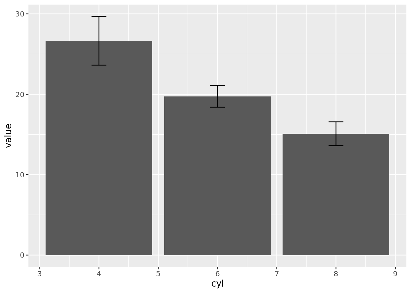
# create MEAN column chart with error bars (using 95% confidence intervals) require(PHEindicatormethods)mtcars%>%filter(!is.na(cyl))%>%group_by(cyl)%>%#use phe_mean()phe_mean(x =mpg, # field name from data containing the values to calculate the means for type ="full", # defines the data and metadata columns to be included in output; can be "value", "lower", "upper", "standard" (for all data) or "full" (for all data and metadata); quoted string; default = "full" confidence =0.95)%>%#required level of confidence expressed as a number between 0.9 and 1# create column chart with error bars (using 95% CI calculated using phe_mean())ggplot(aes(cyl, value))+geom_col(na.rm =TRUE)+geom_errorbar(aes(ymin =lowercl, ymax =uppercl), position ="dodge", width =0.25)
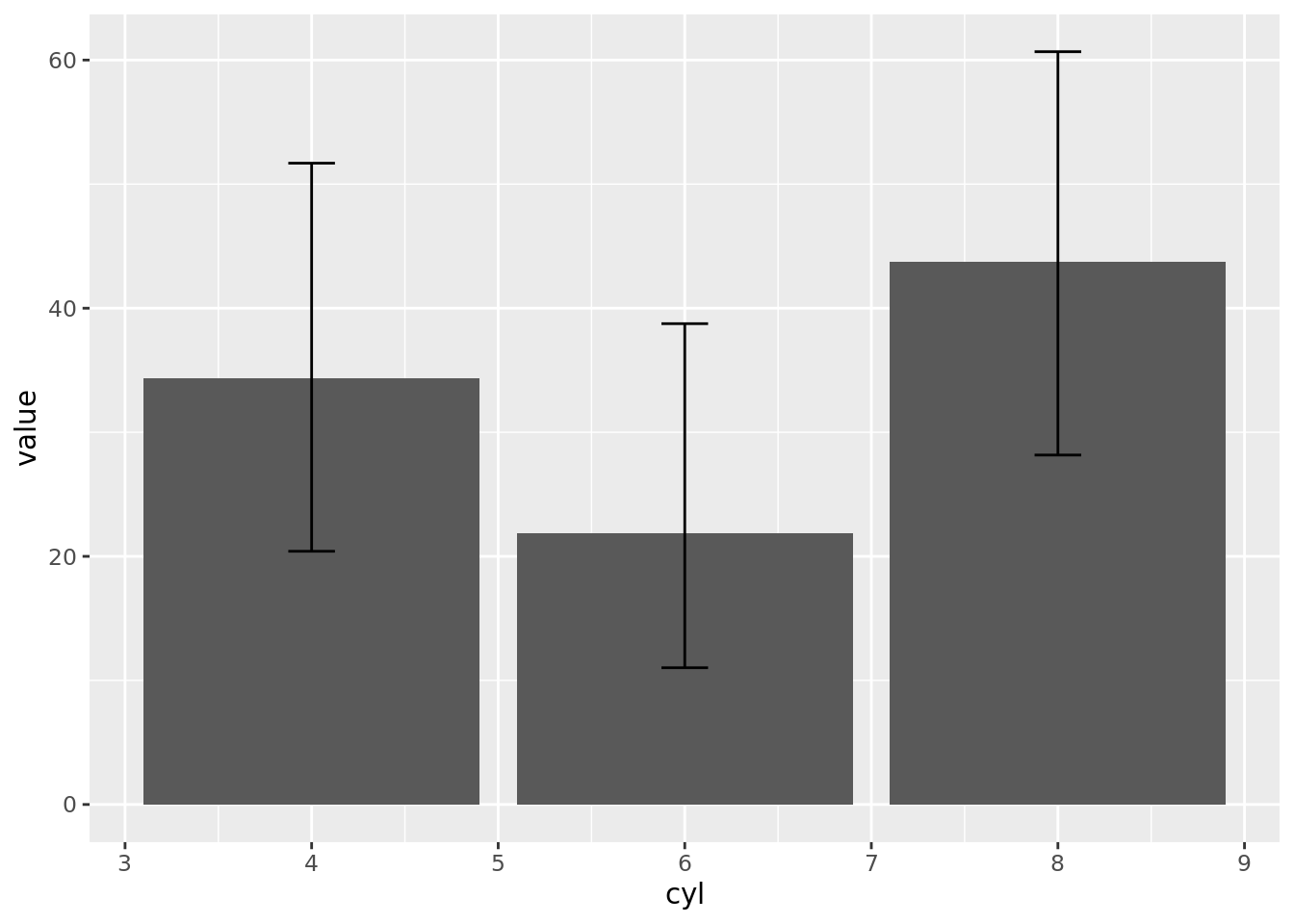
# create PROPORTION column chart with error bars (using 95% confidence intervals) require(PHEindicatormethods)mtcars%>%group_by(cyl)%>%summarise(n =n(), sum =sum(n))%>%mutate(sum =sum(n))%>%# phe_proportion()phe_proportion(x =n, # numerator n =sum, # denominator type ="full", # defines the data and metadata columns to be included in output; can be "value", "lower", "upper", "standard" (for all data) or "full" (for all data and metadata); quoted string; default = "full" confidence =0.95, # required level of confidence expressed as a number between 0.9 and 1 multiplier =100)%>%# the multiplier used to express the final values (eg 100 = percentage); numeric; default 1# create column chart with error bars (using 95% CI calculated using phe_proportion())ggplot(aes(cyl, value))+geom_col(na.rm =TRUE)+geom_errorbar(aes(ymin =lowercl, ymax =uppercl), position ="dodge", width =0.25)
I hope that the code, above, helps a few colleagues of mine across the NHS, in some small way.
Thank you, again, to all members of the NHS R Community, for all your help. Particular thanks go to everyone who has helped me, to date, on the NHS R Community’s Slack channel.
Comments (3)
Chuck Burks
5 January 2022
I used to use a function like that, then I realized that I could get a function for standard error through the FSA package, FSA::se(). Arguments can be made either way; why reinvent the wheel vs. why load a large package to avoid writing one function.
Qin Zeng
5 January 2022
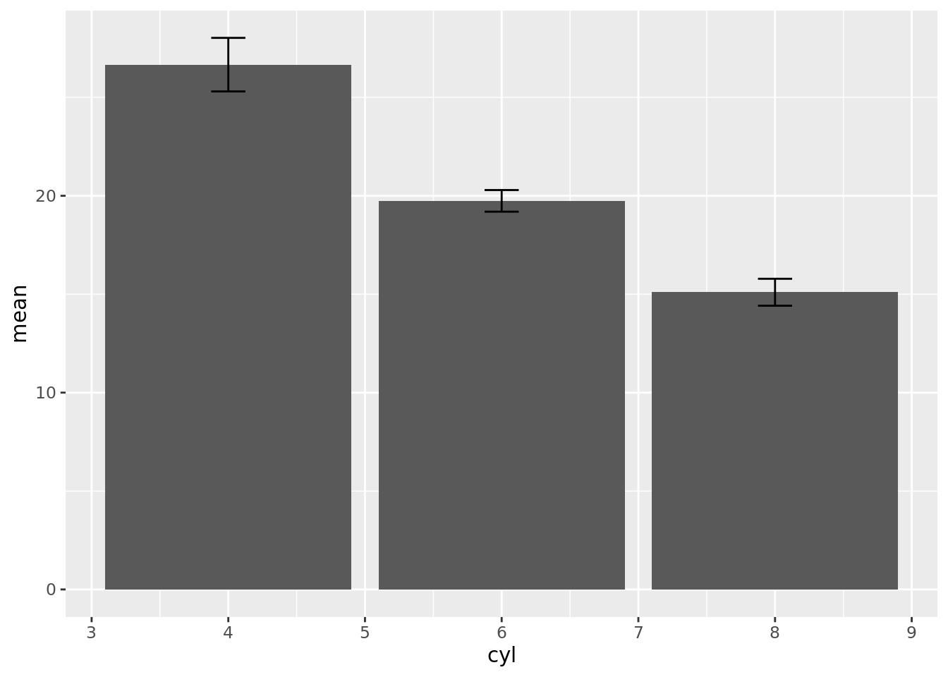
This works out about the same: mtcars %>% group_by(cyl) %>% summarise_at(vars(mpg), funs(n(), mean, min, median, max, sd, stderr)) %>% ggplot(aes(cyl, mean))+ geom_col(na.rm = TRUE)+ geom_errorbar(aes(ymin = mean-stderr, ymax = mean+stderr), position = "dodge", width = 0.25)
Stephen
6 January 2022
Two suggestions: mtcars %>% group_by(cyl) %>% summarise(n = n(), sum = sum(n)) %>% mutate(sum = sum(n)) is more easily said as mtcars %>% count(cyl) %>% mutate(sum = sum(n)) Qin, your sequence is better as mtcars %>% group_by(cyl) %>% summarise(n(), across(mpg, c(mean, min, median, max, sd, stdeQi, in modern dplyr (summarise_at is deprecated)

Comments (3)
Chuck Burks
5 January 2022
I used to use a function like that, then I realized that I could get a function for standard error through the FSA package,
FSA::se(). Arguments can be made either way; why reinvent the wheel vs. why load a large package to avoid writing one function.Qin Zeng
5 January 2022
This works out about the same:
mtcars %>% group_by(cyl) %>% summarise_at(vars(mpg), funs(n(), mean, min, median, max, sd, stderr)) %>% ggplot(aes(cyl, mean))+ geom_col(na.rm = TRUE)+ geom_errorbar(aes(ymin = mean-stderr, ymax = mean+stderr), position = "dodge", width = 0.25)Stephen
6 January 2022
Two suggestions:
mtcars %>% group_by(cyl) %>% summarise(n = n(), sum = sum(n)) %>% mutate(sum = sum(n))is more easily said asmtcars %>% count(cyl) %>% mutate(sum = sum(n))Qin, your sequence is better as mtcars %>% group_by(cyl) %>% summarise(n(), across(mpg, c(mean, min, median, max, sd, stdeQi, in modern dplyr (summarise_at is deprecated)