Authors

Muhammad Faisal

Gary Hutson

Published

April 22, 2021

Modified

July 12, 2024

I recently came across a term synthetic data. I start wondering what does it mean? I found that it is different from the dummy data, but in what ways and how is it different, I began to wonder?

I become curious to find out more about it, as nowadays it is difficult to get hold of healthcare data (that is., NHS). The most prominent issues seem to link to data governance and access, as this information is personal sensitive data.

I investigated methods for creating ‘synthetic data’ as a tool that might help to develop better prediction models, as data could be available for a much larger pool of people, who can tackle these data governance and other challenging healthcare issues.

What is Synthetic data?

The goal is to generate a data set which contains no real units, therefore safe for public release and retains the structure of the data.

In other words, one can say that synthetic data contains all the characteristics of original data minus the sensitive content.

Synthetic data is generally made to validate mathematical models. This data is used to compare the behaviour of the real data against the one generated by the model.

How we generate synthetic data?

The principle is to observe real-world statistic distributions from the original data and reproduce fake data by drawing simple numbers.

Consider a data set with p variables. In a nutshell, synthesis follows these steps:

  1. Take a simple random sample of x1,obs and set as x1,syn

  2. Fit model f(x2,obs|x1,obs) and draw x2,syn from f(x2,syn|x1,syn)

  3. Fit model f(x3,obs|x1,obs , x2,obs ) and draw x3,syn  from f(x3,syn|x1,syn , x2,syn )

  4. And so on, until f(xp,syn|x1,syn , x2,syn , … , xp-1,syn)

Fitting statistical models to the original data and generating completely new records for public release.
Joint distribution f(x1, x2, x3, …, xp) is approximated by a set of conditional distributions f(x2|x1).

For instance, we have the following original (real) data.

tibble::tribble(
      ~sex,                   ~edu, ~age, ~depress,
  "FEMALE",   "VOCATIONAL/GRAMMAR",  57L,       6L,
    "MALE",   "VOCATIONAL/GRAMMAR",  20L,       0L,
  "FEMALE",   "VOCATIONAL/GRAMMAR",  18L,       0L,
  "FEMALE", "PRIMARY/NO EDUCATION",  78L,      16L,
  "FEMALE",   "VOCATIONAL/GRAMMAR",  54L,       4L,
    "MALE",            "SECONDARY",  20L,       5L,
  "FEMALE",            "SECONDARY",  39L,       2L,
    "MALE",            "SECONDARY",  39L,       4L,
  "FEMALE",            "SECONDARY",  43L,       0L,
  "FEMALE",            "SECONDARY",  63L,       6L
  )
# A tibble: 10 × 4
   sex    edu                    age depress
   <chr>  <chr>                <int>   <int>
 1 FEMALE VOCATIONAL/GRAMMAR      57       6
 2 MALE   VOCATIONAL/GRAMMAR      20       0
 3 FEMALE VOCATIONAL/GRAMMAR      18       0
 4 FEMALE PRIMARY/NO EDUCATION    78      16
 5 FEMALE VOCATIONAL/GRAMMAR      54       4
 6 MALE   SECONDARY               20       5
 7 FEMALE SECONDARY               39       2
 8 MALE   SECONDARY               39       4
 9 FEMALE SECONDARY               43       0
10 FEMALE SECONDARY               63       6

We can generate synthetic data using the algorithm described above.

tibble::tribble(
      ~sex,                       ~edu, ~age, ~depress,
    "MALE",     "PRIMARY/NO EDUCATION",  81L,      11L,
  "FEMALE",                "SECONDARY",  75L,       9L,
  "FEMALE",       "VOCATIONAL/GRAMMAR",  43L,       6L,
  "FEMALE",       "VOCATIONAL/GRAMMAR",  65L,       3L,
    "MALE", "POST-SECONDARY OR HIGHER",  17L,       3L,
    "MALE",                "SECONDARY",  39L,       3L,
    "MALE",                "SECONDARY",  35L,       1L,
  "FEMALE",       "VOCATIONAL/GRAMMAR",  35L,       2L,
    "MALE", "POST-SECONDARY OR HIGHER",  38L,       0L,
    "MALE",       "VOCATIONAL/GRAMMAR",  25L,       0L
  )
# A tibble: 10 × 4
   sex    edu                        age depress
   <chr>  <chr>                    <int>   <int>
 1 MALE   PRIMARY/NO EDUCATION        81      11
 2 FEMALE SECONDARY                   75       9
 3 FEMALE VOCATIONAL/GRAMMAR          43       6
 4 FEMALE VOCATIONAL/GRAMMAR          65       3
 5 MALE   POST-SECONDARY OR HIGHER    17       3
 6 MALE   SECONDARY                   39       3
 7 MALE   SECONDARY                   35       1
 8 FEMALE VOCATIONAL/GRAMMAR          35       2
 9 MALE   POST-SECONDARY OR HIGHER    38       0
10 MALE   VOCATIONAL/GRAMMAR          25       0

We can compare the distribution of original data with synthetic data as follows:

Comparison bar charts for sex, edu, age and depress

These charts were created using the shiny app

National early warning score (NEWS) example in R:

library(NHSRdatasets)
library(dplyr)

df <- NHSRdatasets::synthetic_news_data

df |> 
  slice_head(n = 10)
# A tibble: 10 × 12
    male   age  NEWS  syst  dias  temp pulse  resp   sat   sup alert  died
   <int> <int> <int> <int> <int> <dbl> <int> <int> <int> <int> <int> <int>
 1     0    68     3   150    98  36.8    78    26    96     0     0     0
 2     1    94     1   145    67  35      62    18    96     0     0     0
 3     0    85     0   169    69  36.2    54    18    96     0     0     0
 4     1    44     0   154   106  36.9    80    17    96     0     0     0
 5     0    77     1   122    67  36.4    62    20    95     0     0     0
 6     0    58     1   146   106  35.3    73    20    98     0     0     0
 7     0    25     4    65    42  35.6    72    12    99     0     0     0
 8     0    69     0   116    56  37.2    90    16    97     0     0     0
 9     0    91     1   162    72  35.5    60    16    99     0     0     0
10     0    70     1   132    96  35.3    67    16    97     0     0     0
      male            age              NEWS             syst      
 Min.   :0.000   Min.   : 17.00   Min.   : 0.000   Min.   : 65.0  
 1st Qu.:0.000   1st Qu.: 60.00   1st Qu.: 1.000   1st Qu.:118.0  
 Median :0.000   Median : 74.00   Median : 2.000   Median :134.0  
 Mean   :0.476   Mean   : 69.65   Mean   : 2.444   Mean   :135.7  
 3rd Qu.:1.000   3rd Qu.: 84.00   3rd Qu.: 4.000   3rd Qu.:150.0  
 Max.   :1.000   Max.   :102.00   Max.   :12.000   Max.   :220.0  
      dias             temp           pulse            resp      
 Min.   : 17.00   Min.   :33.10   Min.   : 40.0   Min.   :10.00  
 1st Qu.: 63.00   1st Qu.:35.80   1st Qu.: 70.0   1st Qu.:16.00  
 Median : 74.00   Median :36.20   Median : 84.0   Median :18.00  
 Mean   : 74.63   Mean   :36.31   Mean   : 85.8   Mean   :18.39  
 3rd Qu.: 84.00   3rd Qu.:36.70   3rd Qu.: 98.0   3rd Qu.:20.00  
 Max.   :124.00   Max.   :40.20   Max.   :200.0   Max.   :43.00  
      sat              sup            alert            died     
 Min.   : 82.00   Min.   :0.000   Min.   :0.000   Min.   :0.00  
 1st Qu.: 95.00   1st Qu.:0.000   1st Qu.:0.000   1st Qu.:0.00  
 Median : 97.00   Median :0.000   Median :0.000   Median :0.00  
 Mean   : 96.38   Mean   :0.123   Mean   :0.071   Mean   :0.07  
 3rd Qu.: 98.00   3rd Qu.:0.000   3rd Qu.:0.000   3rd Qu.:0.00  
 Max.   :100.00   Max.   :1.000   Max.   :3.000   Max.   :1.00  

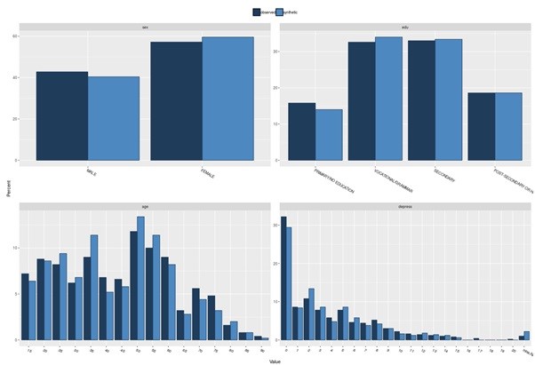
Generate the synthetic NEWS data using synthpop R package

library(synthpop)

syn_df <- syn(df, seed = 4321)
Warning: In your synthesis there are numeric variables with 5 or fewer levels: male, sup, alert, died.
Consider changing them to factors. You can do it using parameter 'minnumlevels'.

Synthesis
-----------
 male age NEWS syst dias temp pulse resp sat sup
 alert died
# synthetic data
syn_df$syn[1:10,]
   male age NEWS syst dias temp pulse resp sat sup alert died
1     1  56    1  126   84 35.7    72   17  98   0     0    0
2     1  50    2  115   84 36.8    94   14  97   0     0    0
3     0  74    6  143   86 36.5    82   21  93   0     0    0
4     1  56    1  122   60 36.3    94   12  98   0     0    0
5     1  52    0  153   89 36.2    78   12  96   0     0    0
6     0  21    2  164   92 35.5    97   20  99   0     0    0
7     0  37    1  101   57 35.6    76   15  98   0     0    0
8     1  81    2  125   74 36.6    71   17  97   0     0    0
9     1  67    5  182  103 37.1    95   18  94   1     0    0
10    1  67    0  160   80 36.2    86   18  98   0     0    0
summary(syn_df$syn) 
      male           age              NEWS             syst      
 Min.   :0.00   Min.   : 17.00   Min.   : 0.000   Min.   : 65.0  
 1st Qu.:0.00   1st Qu.: 60.00   1st Qu.: 1.000   1st Qu.:118.0  
 Median :0.00   Median : 74.00   Median : 1.000   Median :135.0  
 Mean   :0.47   Mean   : 69.99   Mean   : 2.414   Mean   :136.2  
 3rd Qu.:1.00   3rd Qu.: 84.00   3rd Qu.: 4.000   3rd Qu.:150.2  
 Max.   :1.00   Max.   :102.00   Max.   :11.000   Max.   :219.0  
      dias            temp           pulse             resp      
 Min.   : 17.0   Min.   :33.10   Min.   : 43.00   Min.   :12.00  
 1st Qu.: 63.0   1st Qu.:35.80   1st Qu.: 70.00   1st Qu.:16.00  
 Median : 74.0   Median :36.20   Median : 83.00   Median :18.00  
 Mean   : 74.6   Mean   :36.26   Mean   : 85.04   Mean   :18.57  
 3rd Qu.: 84.0   3rd Qu.:36.70   3rd Qu.: 97.00   3rd Qu.:20.00  
 Max.   :124.0   Max.   :40.20   Max.   :200.00   Max.   :43.00  
      sat              sup            alert            died      
 Min.   : 82.00   Min.   :0.000   Min.   :0.000   Min.   :0.000  
 1st Qu.: 95.00   1st Qu.:0.000   1st Qu.:0.000   1st Qu.:0.000  
 Median : 97.00   Median :0.000   Median :0.000   Median :0.000  
 Mean   : 96.45   Mean   :0.125   Mean   :0.059   Mean   :0.062  
 3rd Qu.: 98.00   3rd Qu.:0.000   3rd Qu.:0.000   3rd Qu.:0.000  
 Max.   :100.00   Max.   :1.000   Max.   :3.000   Max.   :1.000  
write.csv("synthetic_news_data.csv")

## "","x"
## "1","synthetic_news_data.csv"

For more discussion about {synthpop} R package http://gradientdescending.com/generating-synthetic-data-sets-with-synthpop-in-r/

Summary

In many ways, synthetic data reflects George Box’s observation that “all models are wrong, but some are useful” while providing a “useful approximation [of] those found in the real world,”

The connection between the clinical outcomes of a patient visits and costs rarely exist in practice, so being able to assess these trade-offs in synthetic data allow for measurement and enhancement of the value of care – cost divided by outcomes.

Synthetic data is likely not a 100% accurate depiction of real-world outcomes, like cost and clinical quality, but rather a useful approximation of these variables. Moreover, synthetic data is constantly improving, and methods like validation and calibration will continue to make these data sources more realistic.

Besides synthetic data used to protect the privacy and confidentiality of set of data, it can be used for testing fraud detection systems by creating realistic behaviour profiles for users and attackers. In machine learning, it can also be used to train and test models. The synthetic data can aid in creating a baseline for future testing or studies such as clinical trial studies.

Dr Muhammad Faisal and Gary Hutson

Back to top

Reuse

CC0

Citation

For attribution, please cite this work as:
Faisal, Muhammad, and Gary Hutson. 2021. “Can We Rely on Synthetic Data to Overcome Data Governance Issue in Healthcare?” April 22, 2021. https://nhs-r-community.github.io/nhs-r-community//blog/can-we-rely-on-synthetic-data-to-overcome-data-governance-issue-in-healthcare.html.